Difference between revisions of "Parameter identifiability example"

Reproducing a test case in BioUML

To reproduce a test case below in the BioUML workbench, go to the Analyses tab in the navigation pane and follow to analyses > Methods > Differential algebraic equations.

Identifiability analysis can be run in two ways:

• to use a pre-created optimization document, double click on Parameter identifiability (optimization);
• for auto-generation of an optimization document using the given settings, double click on Parameter identifiability (table).

Parameter identifiability (optimization)

Definition of the method parameters can be found here.

For our example, we used a test case optimization created for the MAP kinase cascade model of Kholodenko [3]. A brief description of this test case is done in the chapter Optimization examples. In the current identifiability analysis, we used the following settings:

• Path to an optimization document in the BioUML repository:
  Optimization = data/Examples/Optimization/Data/Documents/test_case_2
• Path to an optimization results:
  Parameter values = data/Examples/Optimization/Data/Simulations/optimization_results_2/optimizationInfo
• The maximum number of steps performed by the analysis for each test variable in one direction:
  Maximum identifiability steps = 50
• As the maximal deviation from the initial objective function value, we considered ten percent of the smallest objective function value (found by the optimization and corresponding to the results in the optimizationInfo table):
  Maximal deviation = 4.2
• A possible path to save results of the analysis:
  Output path = data/Collaboration/Demo/Data/Temp/Identifiability results (for test_case_2)

After you click the Run button and the calculations are finished, you will see a result table that includes information on all fitting parameters of the optimization: parameter names (the column "Name"), start values ("Value"), values improved by the analysis ("Estimated value", if these values are equal to the start values, the analysis could not improve the solution of the optimization problem, i.e. started with the best solution), objective function values for the estimated values ("Objective function value"), and links to images, showing the identifiability profile of parameters ("Plot path"):

Clicking on any plot path link will open a new tab with the identifiability profile of the corresponding parameter:

Ready analysis results can be found in the folder:

data/Examples/DAE models/Data/Parameter Identifiability

Parameter identifiability (table)

Definition of the method parameters can be found here.

To get results described above, firstly set the following options:

• Path to a diagram utilized in the test_case_2 optimization:
  Diagram = data/Examples/Optimization/Data/Diagrams/diagram_2
• Path to a table with the same fitting parameters as in the test_case_2 optimization:
  Parameters table = data/Examples/DAE models/Data/Tables/Parameter identifiability (table)/Parameters table
  As the start values (the column "Val"), this table contains the best solution of the optimization problem: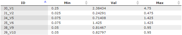
  
  
  
  
• Path to a table with experimental data:
  Observables table = data/Examples/DAE models/Data/Tables/Parameter identifiability (table)/Observables table
  Column names in the table must have the same identifiers as the corresponding entities in the model:
  
  
  
• Name of the time column in the Observbles table:
  Time column = time
• The maximum number of steps performed by the analysis for each test variable in one direction:
  Maximum identifiability steps = 50
• The maximal deviation from the initial objective function value is the same as in the example above:
  Maximal deviation = 4.2
• Optimization method parameters (the same as in the test_case_2 optimization):
  Optimization method name = Particle swarm optimization
  Number of itirations = 200
  Number of particles = 50
• A possible path to save results of the analysis:
  Output path = data/Collaboration/Demo/Data/Temp/Identifiability results (for diagram_2)

After setting these options, your workspace will look like this:

Then click on the phrase "Show expert options":

And additionally set the options for complete coincidence with the optimization problem test_case_2:

• The method to estimate the objective function weights:
  Weight method = Edited
• Path to a table defining the required weights:
  Weights table = data/Examples/DAE models/Data/Tables/Parameter identifiability (table)/Weights table
  
  
  
  
• Name of the column with weights in the Weights table:
  Weight column = Weights

To start the analysis, click on the Run button. The results table is similar to the one obtained from the analysis using the optimization document.

Interpretation of results

In our example, we received the following identifiability profiles:

Identifiability profiles for parameters J0_V1, J1_V2, J4_V5, J8_V9 cross the threshold of a given deviation from the initial objective function value in both directions. Therefore, the analysis defined these variables as identifiable. The identifiability profiles for parameters J5_V6 and J9_V10 cross the threshold in only one direction, so the analysis determined these parameters as partially non-identifiable. However, it should be noted that the resulting J5_V6 value in the optimization problem is equal to the upper bound of the given feasible region.

Other possible profiles

References

1. Raue A, Kreutz C, Maiwald T, Bachmann J, Schilling M, Klingmüller U, Timmer J (2009) Structural and practical identifiability analysis of partially observed dynamical models by exploiting the profile likelihood. Bioinformatics, 25(15):1923–1929.
2. Raue A, Becker V, Klingmüller U, Timmer J (2010) Identifiability and observability analysis for experimental design in nonlinear dynamical models. Chaos, 20(4):045105.
3. Kholodenko BN (2000) Negative feedback and ultrasensitivity can bring about oscillations in the mitogenactivated protein kinase cascades. European Journal of Biochemistry, 267(6):1583–1588.