Difference between revisions of "Optimization examples"
(→Creation of an optimization document) |
|||
| (128 intermediate revisions by one user not shown) | |||
| Line 1: | Line 1: | ||
| − | + | <font size=3> | |
| − | Here we give some examples of | + | Here we give some examples of the [[BioUML]] usage for solving the problem of parameter estimation applied to the models of biochemical pathways. |
| + | For details about creation your oun optimization document in BioUML, see the chapter [[Optimization document]]. All information about the optimization methods implemented in BioUML is done in the chapter [[Optimization problem]]. | ||
| − | == | + | ==Testing the convergence rate of the optimization methods== |
| − | + | <ul> | |
| + | <li>'''Optimization document''': ''data'' > ''Examples'' > ''Optimization'' > ''Data'' > ''Documents'' > ''test_case_1A''</li> | ||
| + | <li>'''Model''': ''data'' > ''Examples'' > ''Optimization'' > ''Data'' > ''Diagrams'' > ''diagram_1A''</li> | ||
| + | <li>'''Experimental data''': ''data'' > ''Examples'' > ''Optimization'' > ''Data'' > ''Experiments'' > ''exp_data_1''</li> | ||
| + | </ul> | ||
| − | |||
| − | + | To analyze a convergence rate of the optimization methods implemented in [[BioUML]] [1], we considered a reaction chain extracted from the model by Neumann et al. [2] and representing activation of caspase-8 triggered by the receptor | |
| − | + | CD95 (APO-1/Fas). | |
| − | + | ||
| − | + | ||
| − | + | ||
| − | + | ||
| − | + | ||
| − | + | ||
| − | + | ||
| − | + | ||
| − | + | ||
| − | + | <table border="0" cellspacing="0" cellpadding="4"> | |
| − | + | <tr> | |
| − | + | <td>[[File:optimization_examples_model_1.png|thumb|The test model of caspase-8 activation]]</td> | |
| + | <td> </td> | ||
| + | <td> | ||
| + | <table border="1" align="center" cellspacing="0" cellpadding="4"> | ||
| + | <tr> | ||
| + | <td>'''ID'''</td> | ||
| + | <td>'''Reactions'''</td> | ||
| + | <td>'''Reaction rates'''</td> | ||
| + | <td>'''Initial values'''</td> | ||
| + | </tr> | ||
| + | <tr> | ||
| + | <td>r1</td> | ||
| + | <td>CD95L + FADD:CD95R → DISC</td> | ||
| + | <td>''k''<sub>1</sub> ⋅ [CD95L] ⋅ [CD95R:FADD]</td> | ||
| + | <td>[CD95L]<sub>0</sub> = 113.220, [CD95R:FADD]<sub>0</sub> = 91.266</td> | ||
| + | </tr> | ||
| + | <tr> | ||
| + | <td>r2</td> | ||
| + | <td>DISC + pro8 → DISC:pro8</td> | ||
| + | <td>''k''<sub>2</sub> ⋅ [DISC] ⋅ [pro8]</td> | ||
| + | <td>[pro8]<sub>0</sub> = 64.477, [DISC]<sub>0</sub> = 0.0</td> | ||
| + | </tr> | ||
| + | <tr> | ||
| + | <td>r3</td> | ||
| + | <td>DISC:pro8 + pro8 → 2 · p43/p41</td> | ||
| + | <td>''k''<sub>3</sub> ⋅ [DISC:pro8] ⋅ [pro8]</td> | ||
| + | <td>[pro8]<sub>0</sub> = 64.477, [DISC:pro8]<sub>0</sub> = 0.0</td> | ||
| + | </tr> | ||
| + | <tr> | ||
| + | <td>r4</td> | ||
| + | <td>2 · p43/p41 → casp8</td> | ||
| + | <td>''k''<sub>4</sub> ⋅ [p43/p41]<sup>2</sup></td> | ||
| + | <td>[p43/p41]<sub>0</sub> = 0.0</td> | ||
| + | </tr> | ||
| + | <tr> | ||
| + | <td>r5</td> | ||
| + | <td>casp8 →</td> | ||
| + | <td>''k''<sub>5</sub> ⋅ [casp8]</td> | ||
| + | <td>[casp8]<sub>0</sub> = 0.0</td> | ||
| + | </tr> | ||
| + | </table> | ||
| + | </td> | ||
| + | </tr> | ||
| + | </table> | ||
| − | + | We performed estimation of parameters using the search space defined as: | |
| − | + | ||
| + | [[File:optimization_examples_formula_1.png]] | ||
| + | |||
| + | where upper bounds were chosen based on the order of magnitude of parameter values proposed in [2]. | ||
| + | |||
| + | Estimation was based on the experimental data obtained by Neumann ''et al''. [2] for procaspase-8 and its cleaved products | ||
| + | p43/p41 and caspase-8. | ||
| + | |||
| + | <table border="1" cellspacing="0" cellpadding="4"> | ||
| + | <tr> | ||
| + | <td>'''Time (min<sup>-1</sup>)'''</td> | ||
| + | <td>'''p43/p41 (nM)'''</td> | ||
| + | <td>'''pro-8 (nM)'''</td> | ||
| + | <td>'''casp-8 (nM)'''</td> | ||
| + | </tr> | ||
| + | <tr> | ||
| + | <td>0.0</td> | ||
| + | <td>0.058</td> | ||
| + | <td>59.963</td> | ||
| + | <td>0.000</td> | ||
| + | </tr> | ||
| + | <tr> | ||
| + | <td>10.0</td> | ||
| + | <td>0.268</td> | ||
| + | <td>57.565</td> | ||
| + | <td>0.041</td> | ||
| + | </tr> | ||
| + | <tr> | ||
| + | <td>20.0</td> | ||
| + | <td>4.760</td> | ||
| + | <td>58.590</td> | ||
| + | <td>0.316</td> | ||
| + | </tr> | ||
| + | <tr> | ||
| + | <td>30.0</td> | ||
| + | <td>8.252</td> | ||
| + | <td>59.422</td> | ||
| + | <td>1.397</td> | ||
| + | </tr> | ||
| + | <tr> | ||
| + | <td>45.0</td> | ||
| + | <td>16.144</td> | ||
| + | <td>48.190</td> | ||
| + | <td>3.520</td> | ||
| + | </tr> | ||
| + | <tr> | ||
| + | <td>60.0</td> | ||
| + | <td>17.021</td> | ||
| + | <td>38.950</td> | ||
| + | <td>3.947</td> | ||
| + | </tr> | ||
| + | <tr> | ||
| + | <td>90.0</td> | ||
| + | <td>15.269</td> | ||
| + | <td>23.502</td> | ||
| + | <td>4.871</td> | ||
| + | </tr> | ||
| + | <tr> | ||
| + | <td>120.0</td> | ||
| + | <td>12.530</td> | ||
| + | <td>13.127</td> | ||
| + | <td>4.878</td> | ||
| + | </tr> | ||
| + | <tr> | ||
| + | <td>150.0</td> | ||
| + | <td>10.335</td> | ||
| + | <td>10.703</td> | ||
| + | <td>4.228</td> | ||
| + | </tr> | ||
| + | </table> | ||
| + | |||
| + | We reviewed solutions obtained by all optimization methods for 100 runs. Each run was based on the generation of 10<sup>7</sup> different guesses. | ||
| + | The best result was obtained by the particle swarm optimization (PSO) and the cellular genetic algorithm (MOCell). Methods SRES, MOCell and PSO found similar solutions. Methods ASA and glbSolve | ||
| + | found other values for parameters ''k''<sub>1</sub> and ''k''<sub>2</sub> showing lower efficiency. | ||
| + | |||
| + | <table border="0" cellspacing="0" cellpadding="4"> | ||
| + | <tr> | ||
| + | <td>[[File:optimization_examples_figure_2.png|thumb|The objective function mean values dynamics for 100 runs. The best value obtained by PSO is marked by the red line.]]</td> | ||
| + | <td> </td> | ||
| + | <td> | ||
| + | '''The best guesses obtained by optimization methods for 100 runs''' | ||
| + | <table border="1" cellspacing="0" cellpadding="4"> | ||
| + | <tr> | ||
| + | <td>'''Parameters'''</td> | ||
| + | <td>'''SRES'''</td> | ||
| + | <td>'''MOCell'''</td> | ||
| + | <td>'''PSO'''</td> | ||
| + | <td>'''ASA'''</td> | ||
| + | <td>'''glbSolve'''</td> | ||
| + | </tr> | ||
| + | <tr> | ||
| + | <td>''k''<sub>1</sub></td> | ||
| + | <td>0.0004691</td> | ||
| + | <td>0.0004611</td> | ||
| + | <td>0.0004277</td> | ||
| + | <td>0.0001028</td> | ||
| + | <td>0.0020576</td> | ||
| + | </tr> | ||
| + | <tr> | ||
| + | <td>''k''<sub>2</sub></td> | ||
| + | <td>0.0002059</td> | ||
| + | <td>0.0002046</td> | ||
| + | <td>0.0002155</td> | ||
| + | <td>0.0007875</td> | ||
| + | <td>0.0001228</td> | ||
| + | </tr> | ||
| + | <tr> | ||
| + | <td>''k''<sub>3</sub></td> | ||
| + | <td>0.0009999</td> | ||
| + | <td>0.0010000</td> | ||
| + | <td>0.0009984</td> | ||
| + | <td>0.0009930</td> | ||
| + | <td>0.0009527</td> | ||
| + | </tr> | ||
| + | <tr> | ||
| + | <td>''k''<sub>4</sub></td> | ||
| + | <td>0.0007915</td> | ||
| + | <td>0.0008225</td> | ||
| + | <td>0.0008419</td> | ||
| + | <td>0.0008117</td> | ||
| + | <td>0.0007790</td> | ||
| + | </tr> | ||
| + | <tr> | ||
| + | <td>''k''<sub>5</sub></td> | ||
| + | <td>0.0325900</td> | ||
| + | <td>0.0336720</td> | ||
| + | <td>0.0334167</td> | ||
| + | <td>0.0334118</td> | ||
| + | <td>0.0313443</td> | ||
| + | </tr> | ||
| + | </table> | ||
| + | </td> | ||
| + | <td> </td> | ||
| + | <td> | ||
| + | '''Values of the objective function for 100 runs''' | ||
| + | <table border="1" cellspacing="0" cellpadding="4"> | ||
| + | <tr> | ||
| + | <td>'''Methods'''</td> | ||
| + | <td nowrap>'''The best value'''</td> | ||
| + | <td nowrap>'''The mean value'''</td> | ||
| + | <td nowrap>'''The worst value'''</td> | ||
| + | </tr> | ||
| + | <tr> | ||
| + | <td>'''PSO'''<sub> </sub></td> | ||
| + | <td>11.787</td> | ||
| + | <td>13.164</td> | ||
| + | <td>14.703</td> | ||
| + | </tr> | ||
| + | <tr> | ||
| + | <td>'''MOCell'''<sub> </sub></td> | ||
| + | <td>12.082</td> | ||
| + | <td>13.484</td> | ||
| + | <td>14.771</td> | ||
| + | </tr> | ||
| + | <tr> | ||
| + | <td>'''SRES'''<sub> </sub></td> | ||
| + | <td>12.466</td> | ||
| + | <td>14.987</td> | ||
| + | <td>18.283</td> | ||
| + | </tr> | ||
| + | <tr> | ||
| + | <td>'''ASA'''<sub> </sub></td> | ||
| + | <td>13.728</td> | ||
| + | <td>15.794</td> | ||
| + | <td>16.610</td> | ||
| + | </tr> | ||
| + | <tr> | ||
| + | <td>'''glbSolve'''<sub> </sub></td> | ||
| + | <td>16.614</td> | ||
| + | <td>16.614</td> | ||
| + | <td>16.614</td> | ||
| + | </tr> | ||
| + | </table> | ||
| + | </td> | ||
| + | </tr> | ||
| + | </table> | ||
| + | |||
| + | ==Testing the computational speed of the optimization methods== | ||
| − | |||
| − | |||
| − | |||
| − | |||
| − | |||
| − | |||
| − | |||
| − | |||
| − | |||
| − | |||
| − | |||
| − | |||
| − | |||
| − | |||
| − | |||
| − | |||
| − | |||
| − | |||
| − | |||
<ul> | <ul> | ||
| − | <li> | + | <li>'''Optimization documents''': ''data'' > ''Examples'' > ''Optimization'' > ''Data'' > ''Documents'' <div></div> (test cases 1A, 1B, 1C, 2, 3) </li> |
| − | '' | + | <li>'''Models''': ''data'' > ''Examples'' > ''Optimization'' > ''Data'' > ''Diagrams'' <div></div> (diagrams 1A, 1B, 1C, 2, 3 for the corresponding test cases) </li> |
| − | </li> | + | <li>'''Experimental data''': ''data'' > ''Examples'' > ''Optimization'' > ''Data'' > ''Experiments'' <div></div> (''exp_data_1'' for the test cases 1A, 1B, 1C; ''exp_data_2'' for the test case 2; ''exp_data_3'' for the test case 3) </li> |
| − | <li> | + | |
| − | '' | + | |
| − | + | ||
| − | </li> | + | |
| − | <li> | + | |
| − | '' | + | |
| − | </li> | + | |
</ul> | </ul> | ||
| − | |||
| − | |||
| − | |||
| − | |||
| − | |||
| − | |||
| − | |||
| − | |||
| − | |||
| − | |||
| − | |||
| − | |||
| − | |||
| − | |||
| − | |||
| − | |||
| − | |||
| − | |||
| − | |||
| + | We tested a computational speed of such optimization methods in BioUML as particle swarm optimization, adaptive simulated annealing, stochastic ranking evolution strategy (SRES), and cellular genetic algorithm. | ||
| + | For this purpose, we used biochemical models with the different number of parameters and species introduced in the following test cases. | ||
| + | Firstly, we derived three models of CD95-induced activation of caspase-8 from the model by Neumann et al. [2] with varying degrees of detail (the test cases 1A, 1B and 1C). | ||
| + | Secondly, we took the test case proposed by Mendes et al. [3] for the MAP kinase cascade model developed by Kholodenko et al. [4] (the test case 2). | ||
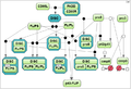
| + | Finally, we tested the model by Bagci et al. [5] representing the mitochondria-depended apoptosis (the test case 3). | ||
| + | |||
| + | As expected, the computational speed for all test cases directly depended on the number of parameters and species in the model. | ||
| + | The greatest computational speed was shown by the method of particle swarm optimization. | ||
| + | The other methods showed about the same speed for running in one core, wherease, for running in several cores, the computational speed of PSO, SRES and MOCell was evidently higher compared to the simulated annealing. | ||
| + | |||
| + | <font size=2> | ||
<gallery> | <gallery> | ||
| − | File: | + | File:optimization_examples_model_1.png|'''Test case 1A''': 7 species and 5 reaction rate parameters. |
| − | File: | + | File:optimization_examples_model_2.png|'''Test case 1B''': 13 species and 10 reaction rate parameters. |
| − | File: | + | File:optimization_examples_model_3.png|'''Test case 1C''': 18 species and 12 reaction rate parameters. |
| − | File: | + | File:optimization_examples_model_4.png|'''Test case 2''': 8 species and 22 reaction rate parameters. |
| − | File: | + | File:optimization_examples_model_5.png|'''Test case 3''': 32 species and 57 reaction rate parameters. |
| − | File: | + | File:optimization_examples_figure_3.png|The number of objective function evaluations per second for the different test cases in BioUML. |
</gallery> | </gallery> | ||
| + | </font> | ||
| + | |||
| + | ==References== | ||
| + | # Kutumova E., Ryabova A., Valeev T., Kolpakov F. BioUML plug-in for nonlinear parameter estimation using multiple experimental data. ''Virtual Biology''. 2013. 1:47-58. | ||
| + | # Neumann L., Pforr C., Beaudouin J., Pappa A., Fricker N., Krammer P.H., Lavrik I.N., Eils R. Dynamics within the CD95 death-inducing signaling complex decide life and death of cells. ''Molecular Systems Biology''. 2010. 6:352. | ||
| + | # Mendes P., Hoops S., Sahle S., Gauges R., Dada J., Kummer U. Computational modeling of biochemical networks using COPASI. ''Methods in Molecular Biology''. 2009. 500:17–59. | ||
| + | # Kholodenko B.N. Negative feedback and ultrasensitivity can bring about oscillations in the mitogenactivated protein kinase cascades. ''European Journal of Biochemistry''. 2000. 267(6):1583–1588. | ||
| + | # Bagci E.Z., Vodovotz Y., Billiar T.R., Ermentrout G.B., Bahar I. Bistability in apoptosis: roles of bax, bcl-2, and mitochondrial permeability transition pores. ''Biophysical Journal''. 2006. 90(5):1546–1559. | ||
| + | |||
| + | </font> | ||
Latest revision as of 12:07, 16 March 2022
Here we give some examples of the BioUML usage for solving the problem of parameter estimation applied to the models of biochemical pathways. For details about creation your oun optimization document in BioUML, see the chapter Optimization document. All information about the optimization methods implemented in BioUML is done in the chapter Optimization problem.
[edit] Testing the convergence rate of the optimization methods
- Optimization document: data > Examples > Optimization > Data > Documents > test_case_1A
- Model: data > Examples > Optimization > Data > Diagrams > diagram_1A
- Experimental data: data > Examples > Optimization > Data > Experiments > exp_data_1
To analyze a convergence rate of the optimization methods implemented in BioUML [1], we considered a reaction chain extracted from the model by Neumann et al. [2] and representing activation of caspase-8 triggered by the receptor
CD95 (APO-1/Fas).
 |
|
We performed estimation of parameters using the search space defined as:
![]()
where upper bounds were chosen based on the order of magnitude of parameter values proposed in [2].
Estimation was based on the experimental data obtained by Neumann et al. [2] for procaspase-8 and its cleaved products p43/p41 and caspase-8.
| Time (min-1) | p43/p41 (nM) | pro-8 (nM) | casp-8 (nM) |
| 0.0 | 0.058 | 59.963 | 0.000 |
| 10.0 | 0.268 | 57.565 | 0.041 |
| 20.0 | 4.760 | 58.590 | 0.316 |
| 30.0 | 8.252 | 59.422 | 1.397 |
| 45.0 | 16.144 | 48.190 | 3.520 |
| 60.0 | 17.021 | 38.950 | 3.947 |
| 90.0 | 15.269 | 23.502 | 4.871 |
| 120.0 | 12.530 | 13.127 | 4.878 |
| 150.0 | 10.335 | 10.703 | 4.228 |
We reviewed solutions obtained by all optimization methods for 100 runs. Each run was based on the generation of 107 different guesses. The best result was obtained by the particle swarm optimization (PSO) and the cellular genetic algorithm (MOCell). Methods SRES, MOCell and PSO found similar solutions. Methods ASA and glbSolve found other values for parameters k1 and k2 showing lower efficiency.
 |
The best guesses obtained by optimization methods for 100 runs
|
Values of the objective function for 100 runs
|
[edit] Testing the computational speed of the optimization methods
- Optimization documents: data > Examples > Optimization > Data > Documents (test cases 1A, 1B, 1C, 2, 3)
- Models: data > Examples > Optimization > Data > Diagrams (diagrams 1A, 1B, 1C, 2, 3 for the corresponding test cases)
- Experimental data: data > Examples > Optimization > Data > Experiments (exp_data_1 for the test cases 1A, 1B, 1C; exp_data_2 for the test case 2; exp_data_3 for the test case 3)
We tested a computational speed of such optimization methods in BioUML as particle swarm optimization, adaptive simulated annealing, stochastic ranking evolution strategy (SRES), and cellular genetic algorithm.
For this purpose, we used biochemical models with the different number of parameters and species introduced in the following test cases.
Firstly, we derived three models of CD95-induced activation of caspase-8 from the model by Neumann et al. [2] with varying degrees of detail (the test cases 1A, 1B and 1C).
Secondly, we took the test case proposed by Mendes et al. [3] for the MAP kinase cascade model developed by Kholodenko et al. [4] (the test case 2).
Finally, we tested the model by Bagci et al. [5] representing the mitochondria-depended apoptosis (the test case 3).
As expected, the computational speed for all test cases directly depended on the number of parameters and species in the model. The greatest computational speed was shown by the method of particle swarm optimization. The other methods showed about the same speed for running in one core, wherease, for running in several cores, the computational speed of PSO, SRES and MOCell was evidently higher compared to the simulated annealing.
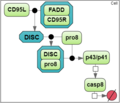
Test case 1A: 7 species and 5 reaction rate parameters.
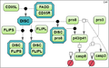
Test case 1B: 13 species and 10 reaction rate parameters.
Test case 1C: 18 species and 12 reaction rate parameters.
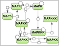
Test case 2: 8 species and 22 reaction rate parameters.
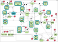
Test case 3: 32 species and 57 reaction rate parameters.
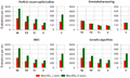
The number of objective function evaluations per second for the different test cases in BioUML.


[edit] References
- Kutumova E., Ryabova A., Valeev T., Kolpakov F. BioUML plug-in for nonlinear parameter estimation using multiple experimental data. Virtual Biology. 2013. 1:47-58.
- Neumann L., Pforr C., Beaudouin J., Pappa A., Fricker N., Krammer P.H., Lavrik I.N., Eils R. Dynamics within the CD95 death-inducing signaling complex decide life and death of cells. Molecular Systems Biology. 2010. 6:352.
- Mendes P., Hoops S., Sahle S., Gauges R., Dada J., Kummer U. Computational modeling of biochemical networks using COPASI. Methods in Molecular Biology. 2009. 500:17–59.
- Kholodenko B.N. Negative feedback and ultrasensitivity can bring about oscillations in the mitogenactivated protein kinase cascades. European Journal of Biochemistry. 2000. 267(6):1583–1588.
- Bagci E.Z., Vodovotz Y., Billiar T.R., Ermentrout G.B., Bahar I. Bistability in apoptosis: roles of bax, bcl-2, and mitochondrial permeability transition pores. Biophysical Journal. 2006. 90(5):1546–1559.