Difference between revisions of "Sensitivity analysis example"

Revision as of 16:07, 11 March 2022

The method description could be found in the section Sensitivity Analysis. Here we give an example of the method application and using in BioUML.

Reproducing a test case in BioUML

To reproduce a test case below in BioUML workbench you first need to go to the Analysis tab in navigation pane and then follow to analyses > Methods > Differential algebraic equations.

After double click on Sensitivity Analysis, a new tab with analysis settings opens.

Select a path to an example diagram:

data/Examples/DAE models/Data/Diagrams/Geva_Zatorsky_2006_Model_I

and a path to save results of analysis, for example:

data/Collaboration/Demo/Data/Temp/Sensitivity Analysis Results

After you click the Run button and the calculations are finished, you can see the results presented in two tables, including scaled and unscaled sensitivities.

Ready analysis results can be found here:

data/Examples/DAE models/Data/Sensitivity Analysis Results

Description of the test case

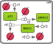
Consider the model of p53 and Mdm2 proteins regulation described by Geva-Zatorsky et al. [1]. The model includes the negative feedback loop in which p53 transcriptionally activates an Mdm2 precursor (pMdm2) representing, for example Mdm2 mRNA, and produces subsequent synthesis of Mdm2. Active Mdm2 increases the degradation rate of p53. The list of the model reactions is done in the table below, where x, y and y₀ denote concentrations of p53, Mdm2 and pMdm2 respectively.

The model of p53 and Mdm2 interactions

ID Reactions Reaction rates r1 → p53 βx r2 -p53 → pMdm2 βy · x r3 pMdm2 → Mdm2 α0 · y0 r4 p53 -Mdm2 → αxy · x · y r5 Mdm2 → αy · y

Assume β_x = 0.3, β_y = 0.4, α₀ = α_y = 0.1 and α_xy = 3.2, and solve the algebraic system:

As a result we obtain the following steady state of the model:

Exploring the unscaled sensitivity of this state to perturbations of parameters β_x, β_y, α₀, α_xy and α_y, we can find the matrix of partial derivatives:

Substituting the values of the investigated parameters, we get:

Scaled sensitivities could be found by the following way:

References

1. Geva-Zatorsky N., Rosenfeld N., Itzkovitz S., Milo R., Sigal A., Dekel E., Yarnitzky T., Liron Y., Polak P., Lahav G., Alon U. Oscillations and variability in the p53 system. Molecular Systems Biology. 2006. V. 2, № 2006.0033.